How to Match Data in Excel

Identifying Records With the MATCH Function

Copy the data lists onto a single worksheet. Excel can work with multiple worksheets within a single workbook, or with multiple workbooks, but you'll find comparing the lists easier if you copy their information onto a single worksheet.

Give each list item a unique identifier. If your two lists don't share a common way to identify them, you may need to add an additional column to each data list that identifies that item to Excel so that it can see if an item in a given list is related to an item in the other list. The nature of this identifier will depend on the kind of data you are trying to match. You will need an identifier for each column list. For financial data associated with a given period, such as with tax records, this could be the description of an asset, the date the asset was acquired, or both. In some cases, an entry may be identified with a code number; however, if the same system is not used for both lists, this identifier may create matches where there are none or ignore matches that should be made. In some cases, you can take items from one list and combine them with items from another list to create an identifier, such as a physical asset description and the year it was purchased. To create such an identifier, you concatenate (add, combine) data from two or more cells using the ampersand (&). To combine an item description in cell F3 with a date in cell G3, separated by a space, you'd enter the formula '=F3&" "&G3' in another cell in that row, such as E3. If you wanted to include only the year in the identifier (because one list uses full dates and the other uses only years), you'd include the YEAR function by entering '=F3&" "&YEAR(G3)' in cell E3 instead. (Do not include the single quotes; they are there only to indicate the example.) Once you've created the formula, you can copy it into all other cells of the identifier column by selecting the cell with the formula and dragging the fill handle over the other cells of the column where you want to copy the formula. When you release your mouse button, each cell you dragged over will be populated with the formula, with the cell references adjusted to the appropriate cells in the same row.

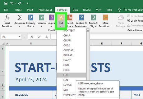
Standardize data where possible. While the mind recognizes that "Inc." and "Incorporated" mean the same thing, Excel doesn't unless you have it re-format one word or the other. Likewise, you may consider values such as $11,950 and $11,999.95 as close enough to match, but Excel won't unless you tell it to. You can deal with some abbreviations, such as "Co" for "Company" and "Inc" for "Incorporated by using LEFT string function to truncate the additional characters. Other abbreviations, such as "Assn" for "Association," may best be dealt with by establishing a data entry style guide and then writing a program to look up and correct improper formats. For strings of numbers, such as ZIP codes where some entries include the ZIP+4 suffix and others don't, you can again use the LEFT string function to recognize and match only the primary ZIP codes. To have Excel recognize numeric values that are close but not the same, you can use the ROUND function to round close values to the same number and match them. Extra spaces, such as typing two spaces between words instead of one, can be removed by using the TRIM function.

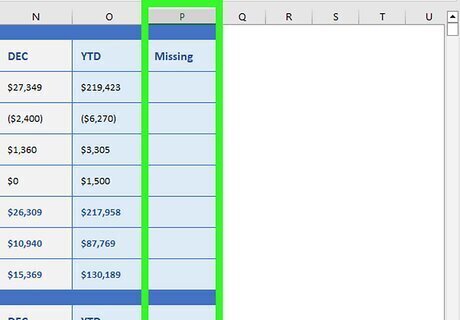
Create columns for the comparison formula. Just as you had to create columns for the list identifiers, you'll need to create columns for the formula that does the comparing for you. You'll need one column for each list. You'll want to label these columns with something like "Missing?"

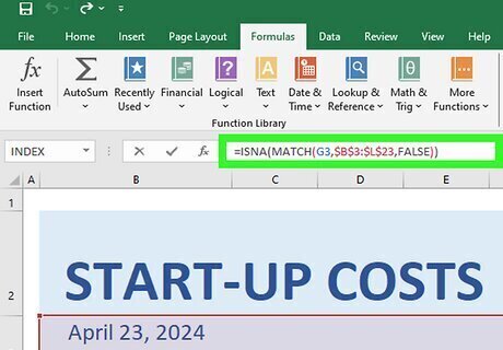
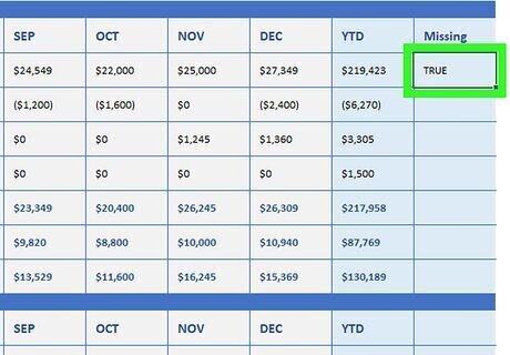
Enter the comparison formula in each cell. For the comparison formula, you'll use the MATCH function nested inside another Excel function, ISNA. The formula takes the form of "=ISNA(MATCH(G3,$L$3:$L$14,FALSE))", where a cell of the identifier column of the first list is compared against each of the identifiers in the second list to see if it matches one of them. If it doesn't match, a record is missing, and the word "TRUE" will be displayed in that cell. If it does match, the record is present, and the word "FALSE" will be displayed. (When entering the formula, do not include the enclosing quotes.) You can copy the formula into the remaining cells of the column the same way you copied the cell identifier formula. In this case, only the cell reference for the identifier cell changes, as putting the dollar signs in front of the row and column references for the first and last cells in the list of the second cell identifiers makes them absolute references. You can copy the comparison formula for the first list into the first cell of the column for the second list. You'll then have to edit the cell references so that "G3" is replaced with the reference for the first identifier cell of the second list and "$L$3:$L$14" is replaced with the first and last identifier cell of the second list. (Leave the dollar signs and colon alone.) You can then copy this edited formula into the remaining cells in the comparison row of the second list.

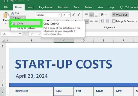
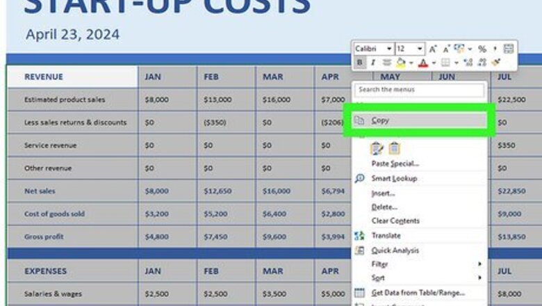
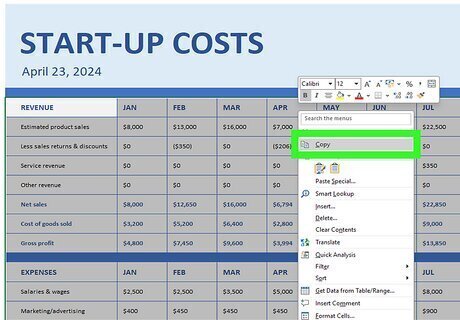
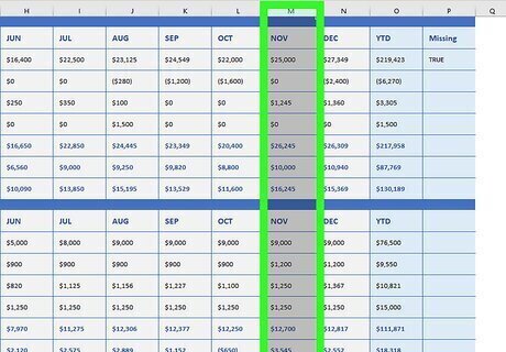
Sort the lists to see non-matching values more easily, if necessary. If your lists are large, you may need to sort them to put all the non-matching values together. The instructions in the substeps below will convert the formulas to values to avoid recalculation errors, and if your lists are large, will avoid a long recalculation time. Drag your mouse over all the cells in a list to select it. Select Copy from the Edit menu in Excel 2003 or from the Clipboard group of the Home ribbon in Excel 2007 or 2010. Select Paste Special from the Edit menu in Excel 2003 or from the Paste dropdown button in the Clipboard group of Excel 2007 or 2010s Home ribbon. Select "Values" from the Paste As list in the Paste Special dialog box. Click OK to close the dialog. Select Sort from the Data menu in Excel 2003 or the Sort and Filter group of the Data ribbon in Excel 2007 or 2010. Select "Header row" from the "My data range has" list in the Sort By dialog, select "Missing?" (or the name you actually gave the comparison column header) and click OK. Repeat these steps for the other list.

Compare the non-matching items visually to see why they don't match. As noted previously, Excel is designed to look for exact data matches unless you set it up to look for approximate ones. Your non-match could be as simple as an accidental transposing of letters or digits. It could also be something that requires independent verification, such as checking to see if listed assets needed to be reported in the first place.

Conditional Formatting With COUNTIF

Copy the data lists onto a single worksheet.

Decide in which list you want to highlight matching or non-matching records. If you want to highlight records in only one list, you'll probably want to highlight the records unique to that list; that is, records that don't match records in the other list. If you want to highlight records in both lists, you'll want to highlight records that do match each other. For the purposes of this example, we'll assume the first list takes up cells G3 through G14 and the second list takes up cells L3 through L14.

Select the items in the list you wish to highlight unique or matching items in. If you wish to highlight matching items in both lists, you'll have to select the lists one at a time and apply the comparison formula (described in the next step) to each list.

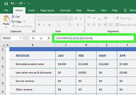
Apply the appropriate comparison formula. To do this, you'll have to access the Conditional Formatting dialog in your version of Excel. In Excel 2003, you do so by selecting Conditional Formatting from the Format menu, while in Excel 2007 and 2010, you click the Conditional Formatting button in the Styles group of the Home ribbon. Select the rule type as "Formula" and enter your formula in the Edit the Rule Description field. If you want to highlight records unique to the first list, the formula would be "=COUNTIF($L$3:$L$14,G3=0)", with the range of cells of the second list rendered as absolute values and the reference to the first cell of the first list as a relative value. (Don't enter the close quotes.) If you want to highlight records unique to the second list, the formula would be "=COUNTIF($G$3:$G$14,L3=0)", with the range of cells of the first list rendered as absolute values and the reference to the first cell of the second list as a relative value. (Don't enter the close quotes.) If you want to highlight the records in each list that are found in the other list, you'll need two formulas, one for the first list and one for the second. The formula for the first list is "=COUNTIF($L$3:$L$14,G3>0)", while the formula for the second list is COUNTIF($G$3:$G$14,L3>0)". As noted previously, you select the first list to apply its formula and then select the second list to apply its formula. Apply whatever formatting you want to highlight the records being flagged. Click OK to close the dialog.