views
Preventing Future Errors
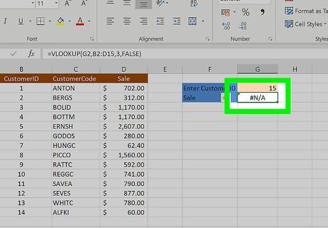
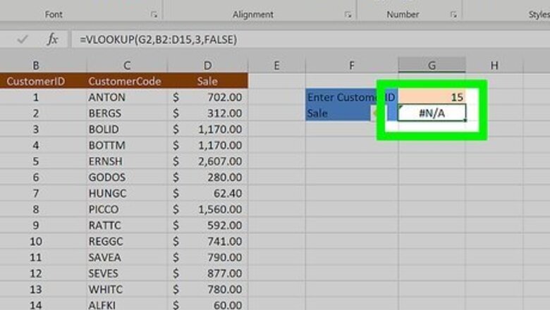
Click on the cell that will contain your main formula. This is the formula that you are trying to manage errors for. Some examples of when you may predict errors are: When you know some referenced data in a VLOOKUP formula might be missing. VLOOKUP will return #N/A when it cannot find the lookup value in the specified array. When you are using a division formula across a referenced dataset, and you know that you may have some missing values in the dividend. Dividing by 0 or a blank cell will result in a #DIV/0! error.
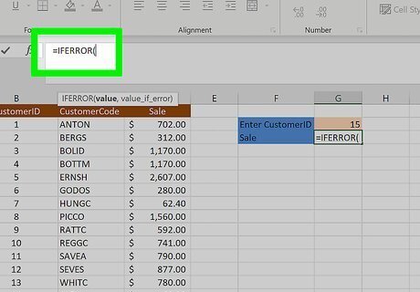
Start typing the IFERROR function. Type the equal sign = followed by IFERROR(. The IFERROR function takes 2 arguments: the value to check for errors and the value to return in place of the error value.
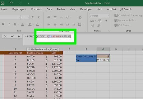
Enter the value that may result in an error. This can be a formula, referenced cell, or expression. Separate this from the next input by typing a comma , after the value.
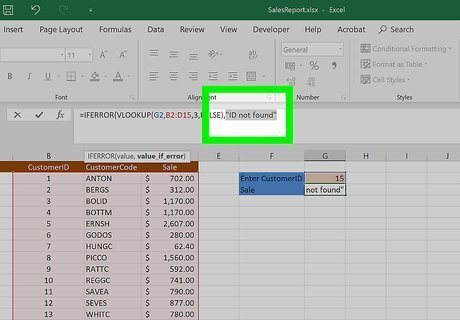
Enter the value that should replace the error. This can be text, a number, another formula, or blank. To use text, make sure you place quotation marks around the text. To replace the error with a blank cell, type "" as this value.
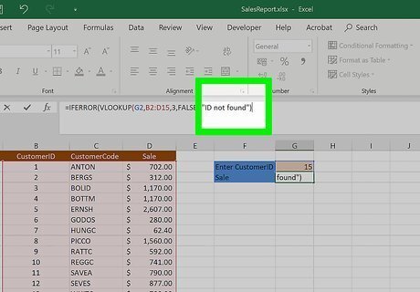
End your function with ). In total, the function should look like IFERROR(value, value_if_error). Some examples of this formula may be: IFERROR(VLOOKUP(F1,A:B,2,FALSE),"missing") would first attempt to look for the value in F1 in column A and return its corresponding value from column B. Excel would then show the word "missing" if it couldn't find F1's value in column B, rather than #N/A. IFERROR(A1/B1,"") would return a blank cell instead of #DIV/0! if B1 was a 0 or blank.
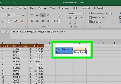
Hit ↵ Enter to finish the formula. Check that it has returned the result you expected.
Managing Existing Errors
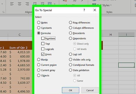
Find errors in your Excel spreadsheet. You can automatically select all errors doing the following: In the Home tab, click Find & Select in the Editing section Select Go To Special…. Select Formulas, then untick everything except Errors. Click OK.
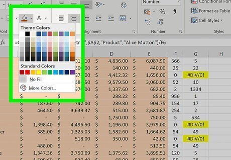
Keep track of the errors. You may want to change the cell color so you can spot them easily on the spreadsheet. To change cell color, click the down arrow next to the Fill Color button while keeping the cells highlighted. This button is found in the Font section in the Home tab. Select a color.
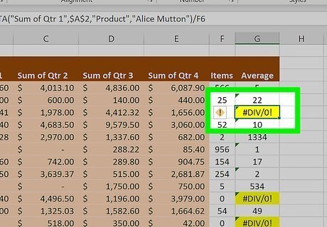
Find an error you want to replace with a value. This shouldn't necessarily be every error you find—some errors may need to be fixed.
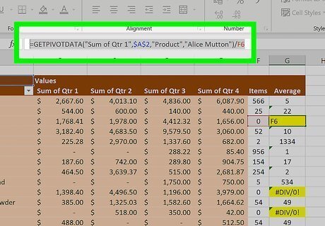
Double-click on the cell to edit the formula. Or you can click the cell, then click into the formula bar at the top to edit.
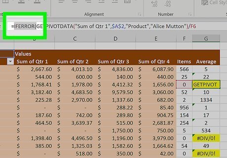
Click your cursor in between the equal sign = and the start of the existing formula. Type IFERROR(.
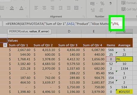
Click your cursor at the end of the existing formula. Enter a comma ,.
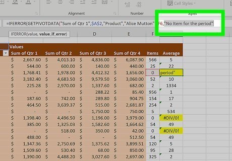
Enter the value that should replace the error. This can be text, a number, another formula, or blank. To use text, make sure you place quotation marks around the text. To replace the error with a blank cell, type "" as this value.
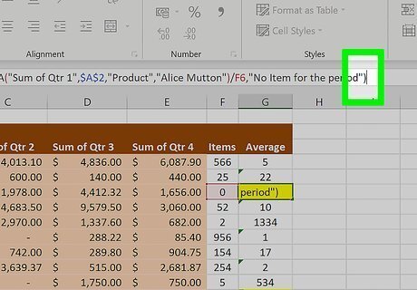
End your function with ). In total, the function should look like IFERROR(value, value_if_error). Some examples of this formula may be: IFERROR(VLOOKUP(C1,A:B,2,FALSE),"missing") would first attempt to look for the value in C1 in column A and return its corresponding value from column B. Excel would then show the word "missing" if it couldn't find C1's value in column B, rather than #N/A. IFERROR(A1/B1,"") would return a blank cell instead of #DIV/0! if B1 was a 0 or blank.
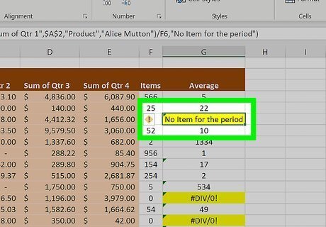
Hit ↵ Enter to finish the formula. Check that it has returned the result you expected.




Comments
0 comment