How to Compare Two Lists in Excel

Using the CountIf Formula

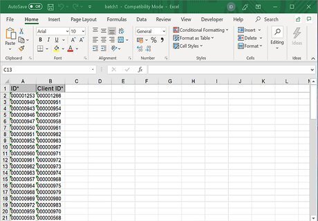
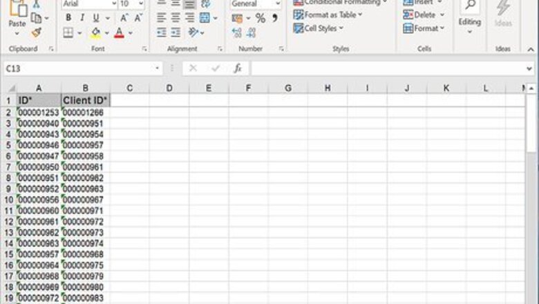
Open the Excel spreadsheet you want to edit. Find the spreadsheet file with the lists you want to compare, and double-click the file to open it in Microsoft Excel.

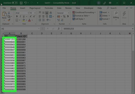
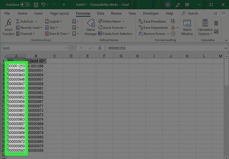
Select your first list. Click the first cell on your first list, and drag your mouse all the way down to the list's last cell to select the entire data range.

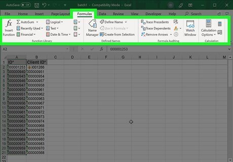
Click the Formulas tab on the toolbar ribbon. You can find this tab above the toolbar at the top of your spreadsheet. It will open your formula tools on the toolbar ribbon.

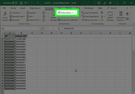
Click Define Name on the toolbar. You can find this option in the middle of the "Formulas" ribbon. It will open a new pop-up window, and allow you to name your list.

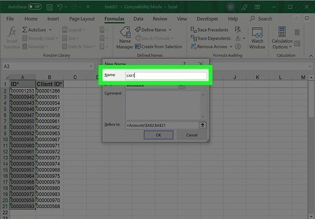
Type List1 into the Name field. Click the text field at the top of the pop-up window, and enter a list name here. You can later use this name to insert your list into the comparison formula. Alternatively, you can give your list a different name here. For example, if this is a list of locations, you can name it "locations1" or "locationList."

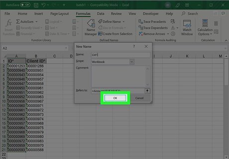
Click OK in the pop-up window. This will confirm your action, and name your list.

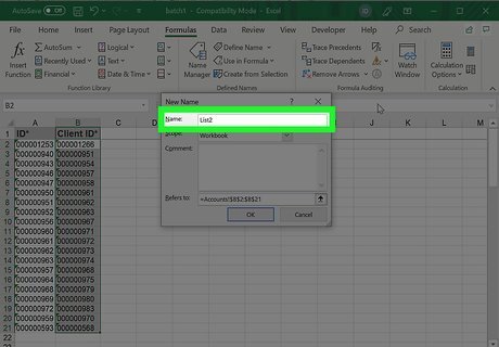
Name your second list as List2. Follow the same steps as the first list, and give your second list a name. This will allow you to quickly use this second list in your comparison formula later. You can give the list any name you want. Make sure to remember or note down the name you give to each of your lists here.

Select your first list. Click the first cell on the first list, and drag down to select the entire data range. Make sure your first list is selected before you start setting up your conditional formatting.

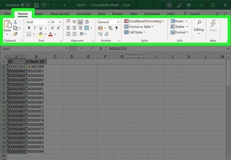
Click the Home tab on the toolbar. This is the first tab in the upper-left corner of the toolbar ribbon. It will open your basic spreadsheet tools on the toolbar.

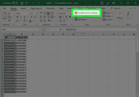
Click Conditional Formatting on the toolbar. This option looks like a tiny spreadsheet icon with some cells highlighted in red and blue. It will open a drop-down menu of all your formatting options.

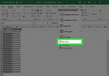
Click New Rule on the drop-down menu. It will open a new pop-up window, and allow you to manually set up a new formatting rule for the selected range.

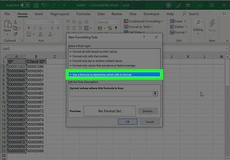
Select the "Use a formula to determine which cells to format" option. This option will allow you to manually type a formatting formula to compare your two lists. On Windows, you'll find it at the bottom of the rule list in the "Select a Rule Type" box. On Mac, select Classic in the "Style" drop-down at the top of the pop-up. Then, find this option in the second drop-down below the Style menu.

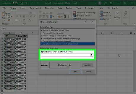
Click the formula field in the pop-up window. You can enter any valid Excel formula here to set up a conditional formatting rule.

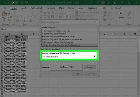
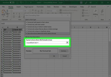
Type =countif(List2,A1)=1 into the formula bar. This formula will scan your two lists, and mark all the cells on your first list that also appear on the second list. Replace A1 in the formula with the number of the first cell of your first list. For example, if the first cell of your first list is cell D5, then your formula will look like =countif(List2,D5)=1. If you gave a different name to your second list, make sure to replace List2 in the formula with the actual name of your own list. Alternatively, change the formula to =countif(List2,A1)=0 if you want to mark the cells that do not appear on the second list.

Type =countif(List1,B1)=1 into the formula bar (optional). If you want to find and mark the cells on your second list that also appear on the first list, use this formula instead of the first one. Replace List1 with the name of your first list, and B1 with the first cell of your second list.

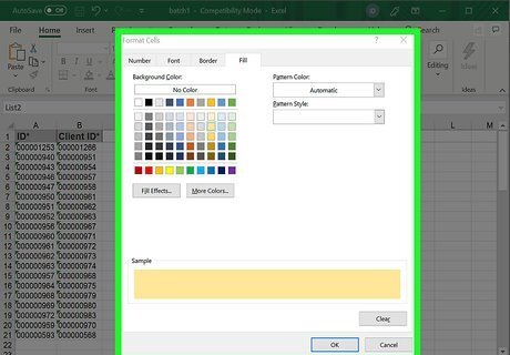
Select a custom format to mark the cells (optional). You can select a custom background fill color and different font styles to mark the cells that your formula finds. On Windows, click the Format button on the bottom-right of the pop-up window. You can select a background color in the "Fill" tab, and font styles in the "Font" tab. On Mac, select a format preset on the "Format with" drop-down at the bottom. You can also select custom format here to manually select a background fill and font styles.

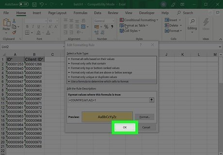
Click OK in the pop-up window. This will confirm and apply your comparison formula. All the cells on your first list that also appear on the second list will be marked with your selected color and font. For example, if you select a light red fill with dark red text, all the recurring cells will turn to this color on your first list. If you use the second formula above, conditional formatting will mark the recurring cells on your second list instead of the first one.

Using the VLookup Formula

Open your Excel spreadsheet. Find the Excel file with the lists you want to compare, and double-click on the file name or icon to open the spreadsheet in Microsoft Excel.

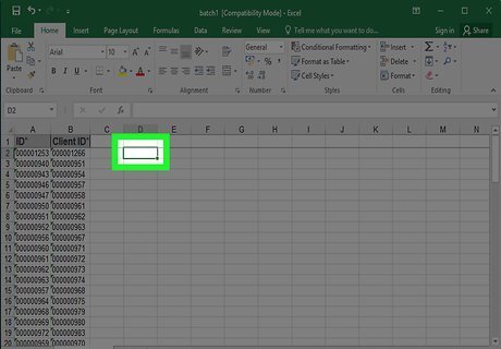
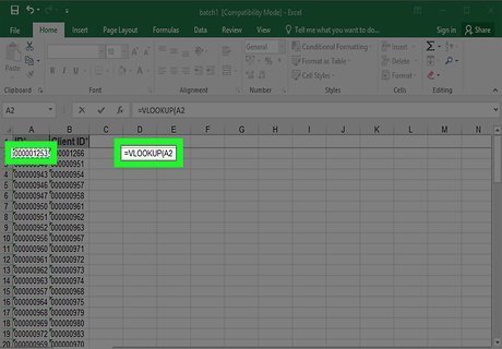
Click the empty cell next to the first item on your second list. Find your second list on the spreadsheet, and click the empty cell next to the first list item at the top. You can insert your VLookup formula here. Alternatively, you can select any empty cell on your spreadsheet. This cell will only make it more convenient for you to see your comparison next to your second list.

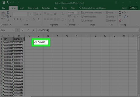
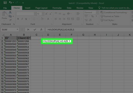
Type =vlookup( into the empty cell. The VLookup formula will allow you to compare all the items on two separate lists, and see if a value is a repeat or new value. Do not close the formula parenthesis until your formula is complete.

Select the first item on your second list. Without closing the formula parenthesis, click the first item on your second list. This will insert your second list's first cell into the formula.

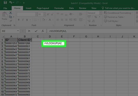
Type a , comma in the formula. After selecting the first cell of your second list, type a comma in the formula. You'll be able to select your comparison range next.

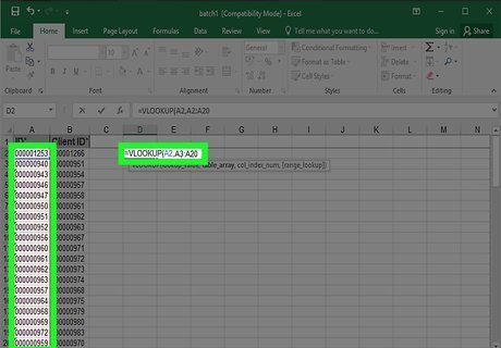
Hold down and select your entire first list. This will insert the cell range of your first list into the second part of the VLookup formula. This will allow you to search the first list for the selected item from your second list (the first item at the top of the second list), and return if it's a repeat or new value.

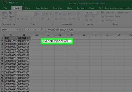
Type a , comma in the formula. This will lock the comparison range in your formula.

Type 1 in the formula after the comma. This number represents your column index number. It will prompt the VLookup formula to search the actual list column instead of a different column next to it. If you want your formula to return the value from the column right next to your first list, type 2 here.

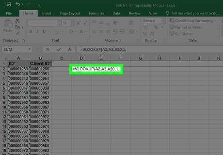
Type a , comma in the formula. This will lock your column index number (1) in the VLookup formula.

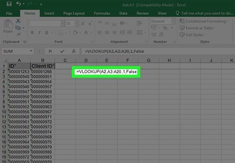
Type FALSE in the formula. This will search the list for an exact match of the selected search item (the first item at the top of the second list) instead of approximate matches. Instead of FALSE you may use 0, it's exactly the same. Alternatively, you can type TRUE or 1 if you want to search for an approximate match.

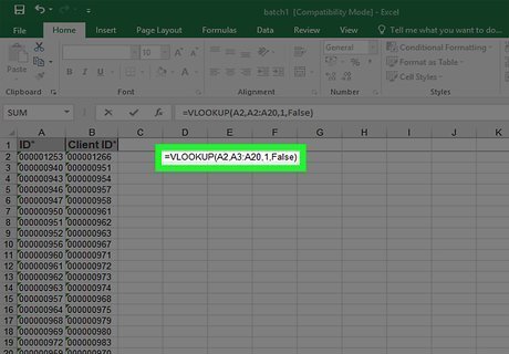
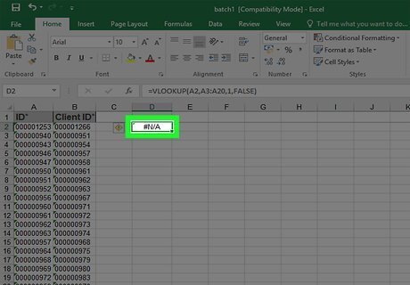
Type ) at the end to close the formula. You can now run your formula, and see if the selected search item on your second list is a repeat or new value. For example, if your second list starts at B1, and your first list goes from cells A1 to A5, your formula will look like =vlookup(B1,$A$1:$A$5,1,false).

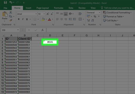
Press ↵ Enter or ⏎ Return on your keyboard. This will run the formula, and search your first list for the first item from your second list. If this is a repeat value, you'll see the same value printed again in the formula cell. If this is a new value, you'll see "#N/A" printed here. For example, if you're searching the first list for "John", and now see "John" in the formula cell, it's a repeat value that comes up on both lists. If you see "#N/A", it's a new value on the second list.

Select your formula cell. After running your formula and seeing your results for the first list item, click on the formula cell to select it.

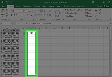
Click and drag down the green dot on the bottom-right of the cell. This will expand your formula cell along the list, and apply the formula to every list item on your second list. This way you can compare every item on your second list to your entire first list. This will search your first list for every item on your second list individually, and show the result next to each cell separately. If you want to see a different marker for new values instead of "#N/A", use this formula: =iferror(vlookup(B1,$A$1:$A$5,1,false),"New Value"). This will print "New Value" for new values instead of "#N/A."